Skip to content
Courses
Blog Posts
Tag:
#valuation
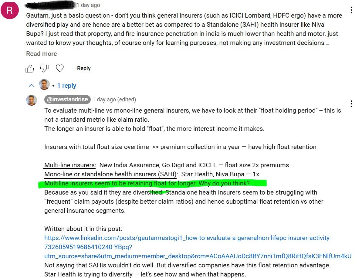
ICICI Lombard, HDFC Ergo Vs Star Health, Niva Bupa
May 27, 2025
How to analyze company earnings con call?
May 27, 2025
How to analyze a general insurance business using Warren Buffett’s method?Learn to spot 🍋
May 27, 2025
“𝙄 𝙨𝙥𝙚𝙣𝙙 𝙢𝙤𝙧𝙚 𝙩𝙞𝙢𝙚 𝙡𝙤𝙤𝙠𝙞𝙣𝙜 𝙖𝙩 𝙗𝙖𝙡𝙖𝙣𝙘𝙚 𝙨𝙝𝙚𝙚𝙩𝙨 𝙩𝙝𝙖𝙣 𝙄 𝙙𝙤 𝙞𝙣𝙘𝙤𝙢𝙚 𝙨𝙩𝙖𝙩𝙚𝙢𝙚𝙣𝙩𝙨. 𝘼𝙣𝙙 𝙒𝙖𝙡𝙡𝙨𝙩𝙧𝙚𝙚𝙩 𝙙𝙤𝙚𝙨 𝙣𝙤𝙩 𝙧𝙚𝙖𝙡𝙡𝙮 𝙥𝙖𝙮 𝙖𝙩𝙩𝙚𝙣𝙩𝙞𝙤𝙣 𝙩𝙤 𝙗𝙖𝙡𝙖𝙣𝙘𝙚 𝙨𝙝𝙚𝙚𝙩𝙨,
May 27, 2025
𝗘𝗻𝗱 𝗼𝗳 𝗮𝗻 𝗲𝗿𝗮!
May 27, 2025
𝗪𝗵𝘆 𝗶𝘀 𝗣/𝗕 𝗮 𝗯𝗲𝘁𝘁𝗲𝗿 𝘃𝗮𝗹𝘂𝗮𝘁𝗶𝗼𝗻 𝗺𝗲𝘁𝗿𝗶𝗰 𝘁𝗵𝗮𝗻 𝗣/𝗘 𝗳𝗼𝗿 𝗕𝗮𝗻𝗸𝘀?
May 27, 2025
Why EV and EV multiples are not a good fit for banks
May 27, 2025
𝗟𝗲𝗮𝗿𝗻 𝗾𝘂𝗶𝗰𝗸 𝗗𝗖𝗙 𝗩𝗮𝗹𝘂𝗮𝘁𝗶𝗼𝗻 𝘂𝘀𝗶𝗻𝗴 𝗶𝗻𝗳𝗼 𝗳𝗿𝗼𝗺 𝘀𝗰𝗿𝗲𝗲𝗻𝗲𝗿.𝗶𝗻
May 27, 2025
𝗡𝗲𝘄 𝗬𝗼𝗿𝗸 🌆 𝗶𝘀 𝗼𝗳𝘁𝗲𝗻 𝗿𝗲𝗳𝗲𝗿𝗿𝗲𝗱 𝘁𝗼 𝗮𝘀 𝘁𝗵𝗲 𝗖𝗼𝗻𝗰𝗿𝗲𝘁𝗲 𝗝𝘂𝗻𝗴𝗹𝗲!
May 27, 2025
𝗛𝗼𝘄 𝘁𝗼 𝗮𝗻𝗮𝗹𝘆𝘇𝗲 𝗮 𝗗𝗔𝗜𝗥𝗬 𝗯𝘂𝘀𝗶𝗻𝗲𝘀𝘀?
May 27, 2025
Previous Page
1
2
3
4
…
6
Next Page
Connect with us
Please enable JavaScript in your browser to complete this form.
Please enable JavaScript in your browser to complete this form.
Name
*
First
Last
Email
*
Message or Name
Comment or Message
Submit
CLOSE