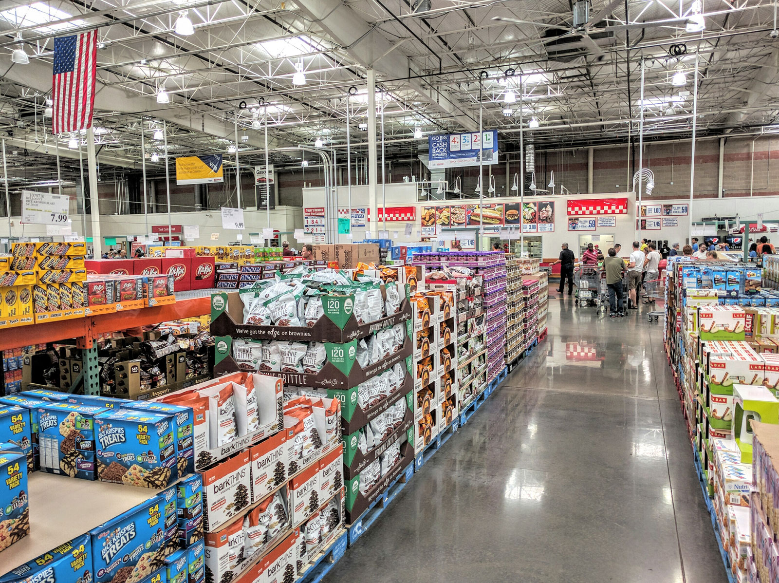
Costco Equity Valuation

Costco Wholesale Corporation (Costco) has a solid business model with a predictable stream of subscription revenue, which constitutes 90% of the net profit.

In the video (embedded below), I have projected out Costco’s financial statements and valued its equity. Although, Costco trades at a P/E of ~36 (amongst the highest in the retail business it operates in), I have found it to be fairly valued.

I have embedded the base excel (without the projections). Please feel free to download and try to model the financial statements and value Costco’s equity if you’d like. Do write to me if you have any questions.

Bandhan Bank IPO Valuation

Credits: businessnewsdaily

Image Credits: businessnewsdaily

The objective is to give a range of fair values to Bandhan Bankโ€™s IPO to help the reader make an informed decision before investing (and the idea is certainly not to predict listing/short-term gains). Relative valuation alone does not really help us when the firm does not have a close second.ย  In our daily life, we like to pay for and invest in tangible things that are priced at fair value, right? And hence the same thing holds true for stocks. In this article, I have tried not to repeat the details about this IPO that are all over the internet. Of course, I have used a lot of data from their Red Herring Prospectus (RHP) and attempted to use some of that key data in making assumptions for the valuation.

I have used the straight forward Excess Return Model (as opposed to FCF methods โ€“ reasons presented in the absolute valuation section) to value the stock of this Financial Services firm BFSL. This method is simple yet very robust for stock valuation Financial Services firms, especially when operational history is limited.

The stock is available at an upper band issue price of Rs. 375.ย  The issue isย overpriced if we assume that the past ROE of 25.55% would be achieved consistently in the future.ย  However, on using excel goal seek functionality which forces the issue price to 375 per share, we arrive at an ROE of 33.80% i.e. if the bank experiences a consistent ROE of 33.80% in the future, it would make the issue fully priced

The below sections shed light on the some of the important qualitative and quantitative factors and then I go on to use those factors in arriving at a range of fair values. You might want to skim straight to the last section on absolute valuation.


The Business model of the entity has transitioned over the years, operating as an NGO in 2001 and then a non-bank finance company (NBFC) before becoming a bank (operations started in Aug 2015), the provision of micro loans to woman has remained a core focus

Competitive advantage โ€“

  • Bandhan Financial Services Limited (BFSL) reaches micro loan customers largely through an extensive network of low cost doorstep service centers (DSC). Low-cost model is demonstrated by our operating cost-to- income ratio was 35.38%
  • The Bank boasts of a differentiated model since on one end they have a stable source of low-cost funding through Current Account and Savings Account (CASA) deposits, which forms 33.22% of their total deposits. On the other end, ~90% of their lending is to microfinance customers which earns them relatively high yields of 18.40% (as of December, 2017)
  • Focus on underbanked and underpenetrated markets allows to meet certain regulatory requirements
  • RBI requires that
    1. Banks locate at least 25% of their banking outlets in what it calls โ€œunbanked ruralโ€ areas. Bandhan Bank has 29.15% of their banking outlets located in unbanked rural areas
    2. Minimum 40% of all lending to be made to Priority Sectors, which includes micro loans. Bandhan has 96.49% of their Gross Advances as Priority Sector Lending (PSL) compliant as of December 31, 2017
  • As per the RHP, “while traditional established commercial banks may not be well suited to targeting unbanked rural areas or providing PSL-compliant lending, and thus see a drag on their profitability and yields. Rather, Bandhan Bank targets unbanked rural area segments by choice, operating a low-cost network designed to cost-effectively and profitably reach these segments”
  • According to CRISIL Research, Eastern and Northeastern India, which are Bandhan’s strongest markets, have the lowest presence of bank branches per capita of any regions in India
  • As of December 31, 2017, percentage of Gross NPAs to Gross Advances (NPAs) was 1.67% of their portfolio. Strong NPA position is largely driven by group-based individual lending model, with focus on income generating loans made to women and lending progressively higher amounts only to members who have built up a track record of good repayment, which taken together have led to low rates of default. Bandhan claims that all micro loan customers areย insured so that if they pass away, their loan balance is paid off in full without their family needing or feeling pressured to repay the loans
  • As at December 31, 2017, capital adequacy ratio was at 24.85% RBI requires a minimum capital adequacy ratio of 13.0% of total risk-weighted assets
  • The Parent entity grew from Indiaโ€™s fourth largest microloan portfolio as of March 31, 2010 to Indiaโ€™s largest microloan portfolio as of March 31, 2012. As of now, over 90% of lending falls under Microfinance, which is a high yielding category

Credit potential in rural India โ€“

  • Although rural India contributes 47% of India’s GDP, its share in total credit outstanding is just 10%, in comparison with 90% for urban India as of fiscal year 2016. This extreme divergence in the share of rural areas in Indiaโ€™s GDP and banking credit is an indicator of the very low penetration of banking in rural areas
  • Buoyed by the Governmentโ€™s sustained efforts to bolster financial inclusion, the number of credit accounts in rural India grew at a 7% CAGR, with the number of deposit accounts rising at an 18% CAGR in fiscal year 2016 from fiscal year 2011. This growth was higher than the 5-years CAGR of 5% in the number of credit accounts, and 14% in the number of deposit accounts in urban India. Notwithstanding, the number of credit and deposit accounts in rural India was almost half that of urban India as of fiscal year 2016
  • 2/3rd of total households are in rural India and the region wise region-wise asymmetry further bolsters the potential for credit growth. Northern and eastern regions have a lower share in total bank credit and deposits. Banking retail credit per capita in the eastern region is the lowest, and is five times lower than the southern region

As per latest RBI data, y-o-y credit growth as of February 2, 2018 was 11.0%

Microcredit sector potential and Bandhan Bankโ€™s current standing โ€“

  • Industry size is pegged to reach ~ INR 1 trillion in next two years driven by rising penetration
  • As per Bharat Micro-finance 2016, MFIN, CRISIL Research (November 2017), the gross loan portfolio (GLP) of MFIs grew at 51% CAGR from fiscal year 2013 to fiscal year 2017. This growth was fuelled largely by the growth in GLP of some large players, such as Janalakshmi Micro-finance, Bharat Financial Inclusion Ltd, Ujjivan Financial Services and Satin Creditcare Network Ltd
  • CRISIL Research expects the MFI loan portfolio growth to be at around 16-18% annually in the next two years, much lower compared with the past four years, as rural areas in well-penetrated states mature and the focus of some top players converting into SFBs shifts towards selling other banking products
  • Banks (including direct and indirect bank lending) account for approximately 60% share of the overall micro-finance credit in India
  • As per he RHP, Bandhan Bank has the largest overall gross micro-banking asset portfolio, with โ‚น213.8 billion as of March 2017, (also counting gross advances, which includes IBPC/Assignment, in the microfinance segment). Amongst the banks (private as well as public), the outstanding loans given by Bandhan Bank is more than three times higher than its closest competitor, the State Bank of India
  • Bandhan Bankโ€™s loan book grew 35% in fiscal year 2017. Highest loan book growth has been registered by Bajaj Finance. Bankโ€™s deposit growth was second only to IDFC Bank. The deposit growth for these two banks was the highest amongst their peers on account of their lower base, as they began to accept deposits only from fiscal year 2016


Cost of funds –ย 

  • Average cost of deposits decreased from 7.72% to 7.09% (annualized) due to an improvement in CASA ratio from 27.22% to 33.22% for the nine months ended December 31, 2016 to the nine months ended December 31, 2017.
  • Increase in CASA i.e. number of deposits led to lesser RBI/inter-bank borrowings (deposits are cheaper than borrowings from RBI/inter-banks), which in turn let to a decrease in overall cost of debt from 7.9% (in FY2017) to 7.24% (annualized) as of December 31, 2017
  • ICICI Bank has a CASA ratio of ~50%, which makes it overall cost of funding to be the lowest (5.3%) in the industry. HDFC and Axis too have a similar CASA and a marginally higher cost of funding. Banks or financial entities which are not into deposits (i.e. โ€œ0โ€ CASA ) typically have higher cost of funding
  • Small Finance Banks with no CASA- AU Small Finance Bank and Janlakshmi Financial Services have high cost of funds of 10.3% and 10.4% respectively. MFIs – Satin CreditCare and Grameen Koota Financial Services cannot have deposits and hence have highest cost of funds @ 13.2%

Absolute Valuation

It is challenging to value BFSL using FCF methods since reinvestment composed of Net CapEx and Working Capital is hard to forecast for financial firms. Moreover, for BFSL it becomes all the more challenging due to the lack of operational history. I was wary of using the Dividend Discount Model (DDM), which again is very similar to FCF, but heavily depends on assumptions around payouts i.e. dividends. BFSL has not obviously paid out any dividends and it does not mention any proposed payout ratios explicitly in the Red Herring Prospectus.

For this valuation, I have used the Excess Return Model, which NYU Stern Prof. Aswath Damodaran has explained brilliantly in his book โ€œInvestment Valuationโ€. This method is relatively straight forward and cuts through layers of complexity. This method is quite intuitive with the idea that it takes the value of both current equity and forecasts of future excess equity returns

Value of Equity = Equity Capital invested currently (including Fresh Issue through IPO) + Present Value of Excess Equity Returns to equity investors;ย 

where Excess Equity Returns = (Return on Equity โ€“ Cost of Equity) * Equity Capital invested

This model requires us to estimate 4 important parameters โ€“

  1. Return on Equity (ROE): BFSL has an annualized ROE of 25.55% as of December 2017
  2. Cost of Equity (COE): Hard to ascertain using CAPM since Beta is not available for an unlisted firm. Moreover, BFSLโ€™s business model is different from a typical listed bank and MFI, which makes it problematic for us to consider the Beta of a peer firm. Nonetheless, we would assume a range of Beta value from 1 to 1.2 to estimate COE

CAPM:ย  COE = Risk Free Rate + (Beta of Stock * Equity Risk Premium)

When Beta = 1: COE = 6.9% +ย  1*5% = 11.9%

When Beta = 1.2: COE = 6.9% + 1.2*5% = 12.9%

Risk Free Rate (RFR) is given to be between 6.7% to 7.1% in the RHP, hence we assume RFR to be 6.9%

  1. Beginning value of Equity: 4446.4 Crores in the beginning of FY2018 as available in the Balance Sheet
  2. Dividend Payout Ratio: No dividends yet obviously. No explicit payout ratio mentioned in the RHP. Payout ratio assumption does not have a significant impact on the valuation using excess return model as it has in DDM. We assume a payout ratio of 5%

To get started, we need to make the judgement as to when BFSL would become a stable growth firm. Because of the under-penetrated microcredit sector and differentiated business model, we canย assume a high growth period of 10 years (stage 1) wherein BFSL sustains its current ROE of 25.55% with a COE) between 11.9 to 12.9%. High growth period is followed by a period of stable growth (stage 2) wherein both return on equity and cost of equity fall and converge to letโ€™s assume 10% i.e. there is no value gained or lost after 10 years, rather excess return generated in stable growth period is 0

The net income each year is computed as the product of ROE and beginning value of equity each year as indicated in the exhibit. Book value of equity each year is estimated each year by adding previous yearโ€™s equity to the retained earnings of the current year


Exhibit โ€“ Excess Return Model

Projected fair value of Rs. 206 per Share on a consistent ROE of 25.55% during the high growth period with Cost of Equity of 11.9%
The fair value reduces to Rs. 190 per Share on increasing Beta to 1.2 (i.e. Cost of Equity of 12.9%)

As we increase Beta, risk increases, and hence value per share further decreases.
Similarly, we can have a range of projected fair values, on changing our estimates of ROE. A 30% ROE throughout the high growth period bumps up the projected fair value to ~ Rs. 287 per share

Using Goal Seek to force the projected fair value to the issue price of Rs. 375 per share revere calculates the ROE to be 33.8% during the high growth period

What this means is that any ROE assumption above 33.8% would make the issue under-priced

No doubt, this method is very simple when compared to the full-blown financial modelling we did in using FCF method of valuation we saw inย the valuation of LT Foodsย . Limited financial history (as presented in the RHP) constrains our ability to work with past data and project it into the future. This again makes the use of other valuation models perhaps untenable since they require a lot of assumptions to be taken. Hence, this makes the straight forward Excess Return Model very powerful to use for Financial Services firms specially when operational history is limited.

About the Author


LT Foods Stock Valuation


Edit (20th Jan 19) – Updated valuation present in https://youtu.be/GlGAZMqMNWY

The objective of this article is to analyze the fundamentals of LT Foods (Daawat Rice) Stock and estimate a fair value per share based on its fundamentals. I have attempted to compare the stock with its peers using certain key financial ratios. I have gone ahead and modeled the financial statements of the firm for the next 5 years and then used the forecasts to ballpark the Free Cash Flow to the Firm (FCFF) in order to arrive at a projected fair value per share

One of the reasons I have chosen this industry is that India is the largest exporter of rice with a 25% share in total exports (in value terms) and also India is the 2nd largest producer and consumer of rice after China (However, China’s share in exports is ~2%). Moreover, globally basmati rice production forms ~1.5% of which India contributes 65-70%. Of late rice firms (with the exception of a few) in India have seen a significant rally and hence I was tempted to analyze one – LT Foods. As per my research and valuation, I have found LT Foods to be overpriced as of this writing (no wonder it is undergoing some correction). Before I begin with the analysis, here is a brief on the firm and its standing amidst its peers –

LT Foods is a leading rice brand in India with a 20% market share in branded basmati rice market. India Business has been growing at a CAGR of 14% over the period FY 2012-17.

It also enjoys leadership position in the US with a 40% market share under brand – Royal with a CAGR of 20% over the last 5 years

Table presents revenue growth and distribution in different geographiesโ€ฉโ€ฉRegion	   Revenue Growth  Revenue Distributionโ€ฉUS	           20%	            28%โ€ฉIndia	           14%	            45%โ€ฉROW	            5%	            15%โ€ฉMiddle East	   10%	            12%โ€ฉ

Out of total revenue of over Rs. 3,300 crore in FY2017, more than Rs. 1,900 crore has been contributed by branded business (i.e. ~60% of the overall top line). Branded business contributes over 71% of the company’s overall volumes and saw a 23% growth in volume terms in FY2017 (and 19% growth in value terms in the same period)

Last year LT foods acquired two brands – Gold Seal Indus Valley and Rozana, from HUL in the Middle East. Besides, they also acquired iconic brand 817 Elephant for American and European market

Table below presents comparison of the fundamentals of this stock with its listed peers (We discuss the comparison of only Chamanlal Setia and KRBL with LT foods in this article. Both Lakhmi energy and Kohinoor have registered negative growth hence we omit them) –

Fundamentally, the stock appears reasonably sound, however, operational efficiency and debt management require improvement –

a.) Inventory Days and Cash Cycle of LT foods (and also KRBL) is quite high in comparison to Chamanlal Setia. Both are measures of the operational efficiency. Cash cycle is defined as the time it takes to convert raw materials into cash. Hence, there is room for improvement in Operations. This view is further bolstered by the slightly lower annual operating margin % vis-a-vis its peers. However, there has been a more or less consistent improvement in operating (EBIDTA) margin over the last 5 years as evident from the exhibit below

b.) Debt to Equity (D/E) ratio of 2.4 seems quite high when compared to its peers. Higher debt ideally should result in a higher ROE, but ROE of LT foods is lower than that of Chamanlal Setia and KRBL. Having said that the company has been able to reduce its D/E from 2.77 in FY2016 to 2.4 in FY2017 as depicted in the exhibit below

c.) Debt has marginally been increasing, so the consistently decreasing D/E can be attributed to increases in retained earnings (share capital remaining the same). High interest on debt adversely affected PAT growth in FY15 and FY16 despite consistently increasing Sales and EBIDTA

Relative Valuation

From a relative valuation standpoint, Chamanlal Setia appears attractive and valuation of KRBL seems stretched. KRBL has the highest P/E, EV/EBIDTA and M Cap/Sales of the lot. Worth noting is that LT Foods M Cap is less than its Sales

Absolute Valuation

Below is an attempt to arrive at the fair value using DCF. There are two methods – Free Cash Flow to Equity (FCFE) and Free Cash Flow to Firm (FCFF).

a.) FCFF is used to estimate Free Cash available to both debt and equity holders. It is arrived at by estimating cash flow generated from operations (CFO), some of which is invested in the purchase and maintenance of fixed assets (Net CapEx) and some of which is used for the working capital (WC). Any cash over and above Net CapEx and WC is available to both debt and equity holders. This is called Free Cash Flow to Firm (FCFF). Present Value of future FCFF is the Enterprise Value (EV). Additionally, removing present debt from EV and dividing by number of shares gives an estimate of fair value

b.) FCFE is used to estimate free cash available for equity holders. We start with forecasting Net Income (NI), some of which goes into Net CapEx and WC and then the left over NI is added along with Net debt issues (or for better understanding, any debt payment is subtracted and new debt issues are added) to arrive at Free Cash Flow available to Equity holders. FCFE is then discounted and divided by the number of shares to determine fair share value

For this valuation, we will use FCFF since FCFE requires forecasting of net debt issues for future years which is difficult for a heavily leveraged company. Another reason is that if net debt issues are high (as is the case with LT Foods), then it increases FCFE beyond Net Income. FCFE estimated in this case if heavily skewed because of inflated debt. Hence, we instead use FCFF in this valuation

Below piece of writing only talks of the key components used in this FCFF valuation

  1. Income Statement Projections
  • Forecasted Net Sales assuming 12.5 % y-o-y sales growth, which is the growth attained in FY2017 over FY2016
  • Expenses to Sales %age assumed to be same as that in FY2017
  • Depreciation & Amortization estimated using useful life of tangible and intangible assets using the straight line method as mentioned in the latest Annual Report. The investment %age (projections) on each PPE component is assumed to be the same as that in FY2017 (Annual Report)

2. Working Capital (WC) Projections โ€“ This schedule is prepared with the purpose to forecast cash flow from operations and use it in FCFF valuation

First, we calculated turnover ratios and using them we calculate average days of sales, inventory and payable outstanding. We then go on to assume that past averages of (receivables, inventory and payables) days outstanding data (albeit with slight improvements) will hold true for future years

For e.g. assuming Days of Sales Outstanding is 45 (days) for future years (47 is the past average. Here we assume slight improvement in Operations resulting in marginal decrease in Days of Sales Outstanding and likewise Receivables and Payables as well)

  • Projected Receivables every future year = (Forecasted Net Sales of that year * Days of Sales Outstanding of that year) / 365
  • Projected Inventory every future year = (Forecasted Net Sales of that year * Days of Inventory Outstanding of that year) / 365
  • Projected Payables every future year = (Forecasted Cost of Sales that year * Days of Payables Outstanding of that year) / 365
  • Net WC = Non Cash Current Assets – Non Cash Current Liabilities
  • Change in (or increase in Net WC) = ( Net WC (in year t) – Net WC (in year t-1) ) / Net WC (in year t-1)

To summarize, we first assume Days of Current Assets and Liabilities Outstanding (based on marginal improvement on past averages) and then use these to forecast Current Assets and Liabilities in future years (by using the formulas mentioned above)

3. CapEx & Depreciation Projections โ€“ This schedule is prepared with the purpose to forecast Net CapEx (= CapEx โ€“ Dep) to use in FCFF valuation

  •  CapEx for future years is estimated using the past average CapEx as a %age of Net Sales. This is a very crude assumption to estimate CapEx. I didn’t come across any specific announcement on future investments by company’s management. In case there is any then I would replace this crude assumption with a more realistic number
  • Depreciation & Amortization estimated using useful life of tangible and intangible assets using the straight line method as mentioned in the latest Annual Report. The investment %age (projections) on each PPE component is assumed to be the same as that in FY2017 (Annual Report)

4. Shareholder Equity Projections โ€“ This is prepared with the purpose to forecast equity, which in turn is used to forecast Return on Capital (ROC)

ROC = Forecasted NI / Forecasted Borrowings and Equity

  • It is difficult to predict future dividend payout ratio (even more so when the annual report does not state out explicitly any target dividend payout). Dividend payout ratio is assumed to be same as in FY2017
  • Ending equity for each year is estimated by using Previous yearโ€™s Equity + Net Income โ€“ Dividends (paid)

2 Stage FCFF valuation

  • This method assumes that growth of the company will continue (stable growth rate) and the return on capital (from 10.8% to 12.1% in 1st 5 years to 10% during stable growth) will be more than cost of capital (9.5% in stable growth period assuming beta goes down from 1.4 to 1.1 and capital structure remaining the same) Another reasonable estimate of the stable growth rate could be the GDP growth rate of the country

FCFF = After Tax Operating Margin OR EBIT(1-T) โ€“ Net CapEx โ€“ Changes in WC

Risk free rate = 6% (the risk free rate is computed as the current yield on 10-year Indian government bond (7.5%) minus the default risk of the Indian government (1.50%)

Stage 1: High Growth Period

  • Since, as per the latest annual report, interest rates (i.e cost of debt) range from 10.70% to 13.15% per annum in 2017 (previous year 10.70% to 13.50% per annum). Here, we have assumed overall cost of debt to be 12% * (1 – Tax Rate)
  • Cost of Equity = 6% + (5% * 1.4) = 13% ; since, Cost of Equity = RFR + (ERP*Beta)
  • Cost of Capital = (12%*(1-0.3)*0.65) + (13% * 0.35) = 10% ; [Pre-Tax Cost of Debt * (1 – T) * Debt as a % of Capital] + [Cost of Equity * Equity as a % of Capital], Debt as a % of Capital is 0.65
  • All Reinvestment Rates in Stage 1 are estimated by calculating forecasted (Net CapEx + change in WC ) as a pecentage of forcasted After Tax Op. Margin or EBIT(1-T)

Stage 2: Stable Growth Period

  • Assumed overall cost of debt to be same as in Stage 1
  • Cost of Equity = 6% + (5% * 1.1) = 11.5% ; assuming beta goes down to 1.1 since the company would be relatively less risky in stable growth period
  • Cost of Capital = (12%*(1-0.3)*0.65) + (11.5% * 0.35) = 9.5% ; Debt as a % of Capital assumed to be same as in Stage 1. Cost of Capital reduces effectively due to reduced cost of equity. Even if cost of debt reduces in stage 2, then lets just assume that beta reduction compensates for any reduction in cost of debt with the overall effect of a reduced cost of capital
  • Since India is a growing economy, we assume growth rate in stable period which is 1% higher than India’s risk free rate. Hence, growth rate = 7% in stable growth period (Stage 2)
  • Reinvestment Rate in Stage 2 estimated using the formula = Assumed Growth Rate (7%) / ROC (9.5%)
  • After Tax Operating Margin after FY2022 = [ EBIT(1-T) in year FY2022 * (1 + assumed stable growth rate 7%)]
  • FCFF = After Tax Operating Margin after FY2022 * ( 1 – Reinvestment Rate in Stage 2)
  • Terminal Value = After Tax Operating Margin after FY2022 / (Cost of Capital 9.5% – assumed stable growth rate 7%)

Enterprise Value (EV) = Net Present Value of FCFF in Stage 1 discounted at Cost of Capital 10% + Terminal Value discounted at Cost of Capital 9.5%

Projected Fair Value Per Share = (EV – Present Debt in FY2017 ) / Number of Shares

Projected Fair Value Per Share is less than the current market price (as on 25th Feb 18) using the 2 stage FCFF model

3 Stage FCFF Valuation

3 Stage Model is typically employed when a high growth period (stage 1) gradually transitions (stage 2) into a stable growth period (stage 3)

With stage 1 and stage 3 assumptions largely remaining the same as in the stage 1 and 2 respectively in the earlier 2-Stage model, we introduce a transition phase (stage 2) with assumed growth rate of 9% (less than that of stage 1 and more than that of stage 3)

Projected Fair Value using this 3 stage method is almost the same as that determined in the earlier 2 stage 2 method

The stock appears slightly overvalued as of this writing (25th Feb 18)

It would be interesting to value ChamanLal Setia using this absolute method since it appears the most attractive relatively

Assuming a more optimistic y-o-y growth (15%) due to acquisition of new brands and also assuming a more than marginal improvement in Operations (10% decrease in inventory and receivables days), fair value jumps to 80 per share. Hence, range of fair value can be pegged to be between 65 – 80

About the Author